
Understanding ResNet: A Milestone in Deep Learning and Image Recognition

ResNet, short for Residual Network, is a convolutional neural network designed to help train very deep networks. Introduced by Kaiming He and colleagues in 2015, its key feature is "skip connections" that allow gradients to flow through the network more effectively, making it possible to train much deeper networks than before. These connections help address the vanishing gradient problem by allowing the network to learn residual functions, stabilizing training and improving performance.
ResNet has been widely applied in various computer vision tasks and comes in several versions, like ResNet-18, ResNet-50, and ResNet-152, indicating the number of network layers. Its innovative approach has significantly influenced deep learning research and applications.
ResNet was a response to the challenges faced by deeper networks. As networks grow deeper, they tend to suffer from vanishing gradients, where the gradient becomes so small it ceases to make a meaningful impact during training. ResNet, through its innovative architecture, tackled this issue head-on, enabling the construction of networks that are deeper yet more efficient than their predecessors.
Let's chat about the magic behind the ResNet architecture, which, frankly, is a bit of a superstar in the neural network realm. At the heart of this ingenious design are these nifty things called residual blocks. Imagine them as the building blocks (quite literally) of ResNet's structure. Now, these aren't just any ordinary blocks; they have a special twist that makes all the difference.
Residual blocks are the cornerstone of ResNet architecture. Each block consists of a few layers of convolutional neural networks (CNNs), usually followed by batch normalization and a ReLU activation function.
Each residual block is a mini-stack of layers from convolutional neural networks (CNNs), which are the bread and butter of image recognition tasks. But ResNet doesn't stop there; it adds a little something extra to the mix. Typically, after the convolutional layers, there's a dash of batch normalization and a sprinkle of ReLU activation function to keep things running smoothly.
Here's where it gets really interesting. ResNet introduces a clever detour in the form of a "skip connection" that literally skips over these layers. Picture this: in a standard CNN setup, an input x gets transformed by some function F(x), which involves all the convolutional operations. But ResNet's residual block shakes things up by making the output F(x) + x instead. This might seem like a small tweak, but it's actually a game changer. It means the block focuses on learning the additional oomph (the residual) it needs to add to the input to get to the desired output. Hence, the name 'Residual Network' – it's all about those extras.
.jpg)
This ingenious setup allows the network to master identity functions effortlessly. Why is this cool? Because it ensures that layers higher up in the network hierarchy can be as good as, or even better than, the ones below. This characteristic is crucial for stacking blocks upon blocks to build deep, deep networks without losing a grip on learning.
By embracing this design, ResNet elegantly sidesteps a common stumbling block in deep learning: as networks get deeper, they often get harder to train due to issues like vanishing gradients. But with residual blocks, ResNet can go deep, really deep, without breaking a sweat. This architectural marvel not only makes it easier to train whoppingly deep networks but also helps in achieving better performance across a wide array of tasks. So, in a nutshell, those little residual blocks are pretty much the unsung heroes of ResNet's success story.
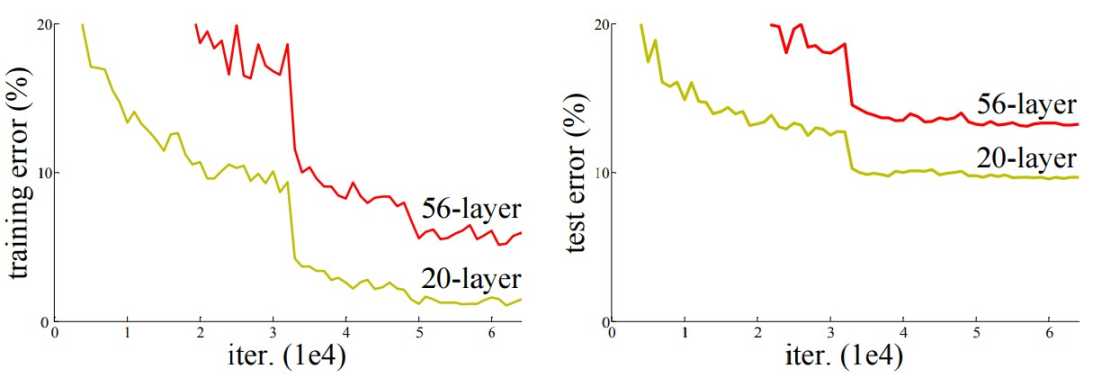
Let's venture into an intriguing phenomenon in the deep learning universe, one that seems a bit counterintuitive at first glance. You'd think that making a neural network larger by adding more layers would be like giving it superpowers, right? More layers, more complexity, and a better knack for understanding the intricacies of data. However, the reality of training deep neural networks often tells a different story.
After piling on a certain number of layers, the performance of these networks doesn't skyrocket as one might hope. Instead, it starts to wobble and even decline. This quirky behavior unveils a gap between what we hope for in theory and what actually happens in practice.
Enter the vanishing gradient problem, a notorious pitfall in the realm of deep learning and data science. This issue is especially bothersome during the training phase of artificial neural networks, where backpropagation and gradient-based learning methods are the norm. The heart of the problem lies in the gradient itself—a critical factor in tweaking the network's weights for better performance.
Imagine the gradient as the network's learning compass, guiding it on how to adjust its weights to get smarter. But what if this compass starts to fade, becoming so faint it's barely noticeable? That's the vanishing gradient problem in a nutshell. When the gradient shrinks to an almost invisible size, the network finds itself in a bind, struggling to update its weights in a meaningful way. It's like trying to find your way in the dark with a nearly extinguished flashlight; you're not going to get very far.
This dilemma is particularly pronounced in deep neural networks. The deeper the network, the longer the journey for the gradient as it travels backward from the output layer to update the weights. With each layer it passes through, the gradient gets progressively smaller, dwindling at an exponential rate. By the time it reaches the earlier layers, it's so weak that it can hardly make an impact. This leaves the early layers of the network in a bit of a limbo, learning at a snail's pace, if at all. The result? The whole training process can hit a roadblock, with the network's performance plateauing or even regressing.
This vanishing gradient issue underscores a paradox in neural network design: bigger (or deeper) isn't always better. It's a reminder that as we push the boundaries of what these networks can do, we also need to navigate around the pitfalls that come with increased complexity.
In the adventurous quest to tackle the deep learning challenges, ResNet emerges as a shining knight, wielding its innovative weapon: skip connections. Picture this: you're navigating through a dense forest (our neural network) and the path (gradient) starts to fade, making it harder to move forward. Then, you find a secret passage (skip connection) that lets you skip some of the most tangled parts of the forest. That's exactly the genius behind ResNet's approach.
These skip connections offer a detour for the gradient during the all-important backpropagation process. Instead of painstakingly winding through every layer of the network, where the gradient can shrink to a whisper, these connections allow the gradient to leapfrog over several layers at a time. It's like finding a shortcut in a maze that keeps you on track towards the exit.
Thanks to this clever architectural design, the gradient keeps its strength, staying robust enough to effectively influence the training process. This means that ResNet can take on much deeper networks without stumbling into the vanishing gradient pitfall. It's a game-changer, pushing the boundaries of what's possible in deep neural network development.
But ResNet's skip connections do more than just solve a technical problem; they open the door to learning from complex data sets more efficiently. By facilitating the training of deeper networks, ResNet significantly amplifies the network's capacity to unravel and learn from the intricacies of vast and complicated data. This advancement isn't just a step forward; it's a giant leap in the field of deep learning, showcasing the power of innovative thinking in overcoming the obstacles that limit progress.
Below is a detailed description of its various architectures:
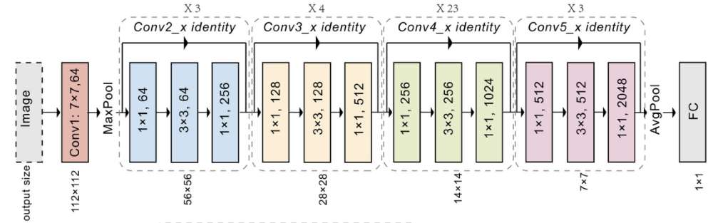
The ResNet family of architectures include different sizes:
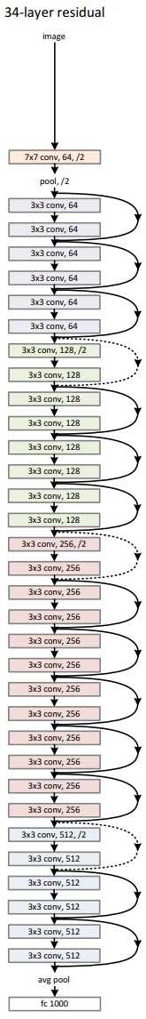
ResNet-34
ResNet's ability to learn deep, complex representations makes it a powerful tool, pushing the boundaries of what's possible in computer vision and related fields.
The Ikomia API allows for easy image classification with ResNet with minimal coding.
To begin, it's important to first install the API in a virtual environment [2]. This setup ensures a smooth and efficient start to using the API's capabilities.
You can also directly charge the notebook we have prepared.

List of parameters:
In this article, we have explored the intricacies of ResNet, a highly effective deep learning model. We've also seen how the Ikomia API facilitates the use of ResNet algorithms, eliminating the hassle of managing dependencies.
The API enhances the development of Computer Vision workflows, offering flexibility in adjusting parameters for both training and testing phases.
To dive deeper, explore how to train ResNet models your custom dataset →
For more information on the API and its capabilities, you can refer to the documentation. Additionally, Ikomia HUB presents a range of advanced algorithms, and Ikomia STUDIO offers an intuitive interface for accessing these functionalities, catering to users who prefer a more graphical approach.


.svg)


